
Introduction
The Naive Bayes algorithm is a simple yet powerful classification technique based on Bayes’ Theorem with a strong assumption of feature independence. It is especially popular in text classification, spam detection, and sentiment analysis because of its high speed and decent accuracy even on relatively small datasets.

Table of Contents
This article dives deep into:
- What Naive Bayes is
- How it works
- Different types
- Pros and cons
- Practical Python implementation
What Is Naive Bayes?
Naive Bayes is a probabilistic classifier that assumes independence among predictors. It calculates the probability of a data point belonging to a particular class and selects the class with the highest probability.
It’s called “naive” because it assumes that all input features are independent of each other—an assumption rarely true in real-world data, but surprisingly effective in practice.
Bayes’ Theorem
The foundation of Naive Bayes is Bayes’ Theorem, which is stated as:
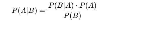
Where:
- P(A|B) = Posterior probability: Probability of hypothesis A given the data B.
- P(B|A) = Likelihood: Probability of data B given that hypothesis A is true.
- P(A) = Prior probability of hypothesis A.
- P(B) = Probability of the data (evidence).
Naive Bayes simplifies this by assuming that all the features are independent given the class.
How Naive Bayes Works
Step-by-Step Breakdown:
- Calculate the prior probabilities for each class.
- For example, if 40% of emails are spam, then P(spam)=0.4P(spam) = 0.4
- Calculate the likelihood of each feature (word/token) given the class.
- For each word in the email: P(word∣spam)
- Multiply all the probabilities together for each class.
- Select the class with the highest probability.
Types of Naive Bayes Classifiers
- Gaussian Naive Bayes
- Used for continuous data that follows a normal distribution.
- Multinomial Naive Bayes
- Ideal for discrete features like word counts or term frequencies.
- Bernoulli Naive Bayes
- Designed for binary/boolean features, like word presence/absence.
Advantages
- Fast and computationally efficient
- Performs well with text classification
- Requires less training data
- Works well even with noisy data
- Easy to implement and understand
Disadvantages
- Assumes feature independence, which is rarely true
- Poor accuracy if this assumption is violated
- Doesn’t handle correlated features well
Real-World Applications
- Spam email filtering
- Sentiment analysis
- Document classification
- Medical diagnosis
- Fraud detection
Python Code: Gaussian Naive Bayes on Iris Dataset
Let’s implement a Gaussian Naive Bayes classifier using scikit-learn.
Step 1: Import Libraries
from sklearn.datasets import load_iris
from sklearn.model_selection import train_test_split
from sklearn.naive_bayes import GaussianNB
from sklearn.metrics import accuracy_score, classification_report
Step 2: Load and Prepare the Data
# Load dataset
iris = load_iris()
X = iris.data
y = iris.target

# Split into training and testing
X_train, X_test, y_train, y_test = train_test_split(X, y, test_size=0.3, random_state=42)
Step 3: Train the Model
# Initialize Gaussian Naive Bayes model
model = GaussianNB()

# Train the model
model.fit(X_train, y_train)
Step 4: Make Predictions and Evaluate
# Predict on test data
y_pred = model.predict(X_test)

# Evaluation
print("Accuracy:", accuracy_score(y_test, y_pred))
print("\nClassification Report:\n", classification_report(y_test, y_pred, target_names=iris.target_names))
Text Classification Example: Multinomial Naive Bayes
Let’s now classify text messages as spam or ham using the Multinomial Naive Bayes model.
Install Dependencies
pip install scikit-learn pandas
Code:
import pandas as pd
from sklearn.feature_extraction.text import CountVectorizer
from sklearn.model_selection import train_test_split
from sklearn.naive_bayes import MultinomialNB
from sklearn.metrics import accuracy_score

# Sample dataset
data = pd.DataFrame({
    'text': [
        'Free money offer now!',
        'Hi, how are you?',
        'Win cash prizes!!!',
        'Let’s have lunch tomorrow',
        'Earn rewards quickly and easily'
    ],
    'label': ['spam', 'ham', 'spam', 'ham', 'spam']
})

# Convert text to features
vectorizer = CountVectorizer()
X = vectorizer.fit_transform(data['text'])
y = data['label']

# Train-test split
X_train, X_test, y_train, y_test = train_test_split(X, y, test_size=0.2, random_state=0)

# Model
clf = MultinomialNB()
clf.fit(X_train, y_train)

# Prediction
y_pred = clf.predict(X_test)

# Accuracy
print("Accuracy:", accuracy_score(y_test, y_pred))
Handling Zero Probabilities: Laplace Smoothing
Naive Bayes can fail when a feature occurs in the test set but not in the training set. This leads to zero probability. To solve this, we use Laplace Smoothing:
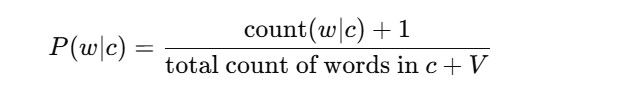
Where VV is the total number of unique words in the training data.
When to Use Naive Bayes
- You have text data (e.g., emails, tweets)
- You need a fast and simple baseline model
- The dataset is small or high-dimensional
When to Avoid
- Features are highly correlated
- You require high precision/recall for sensitive tasks
- You have complex relationships between variables
Conclusion
Naive Bayes is a foundational algorithm in machine learning with broad applications in natural language processing, spam detection, and more. Despite its naive assumption of feature independence, it performs remarkably well in many real-world tasks. Its ease of implementation, speed, and interpretability make it a go-to model for many ML practitioners.
Related Read
K-Nearest Neighbors in sklearn
1 thought on “Naive Bayes Algorithm in Machine Learning”